Conditonal Probability
Let us start with a graphical introduction to the notion of conditional probability 1. Imagine you are throwing darts, and the darts uniformly hit the rectangular dartboard below.
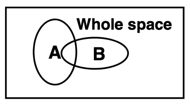
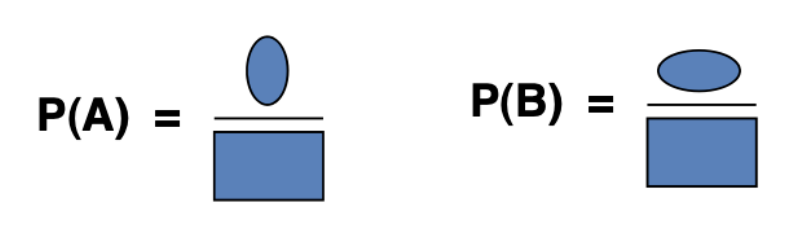
The dark board has two oval shaped pieces of paper labeled \(A\) and \(B\). We can graphically convey the probability of hitting \(A\) and the probability of hitting \(B\) with the images below.
And we can also talk about the probability of hitting \(A\) and \(B\), which is often written as \(A \cap B\), as the image below.
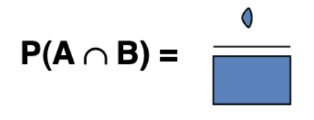
In both cases the denominator is the full entire sample space \(\Omega\) (the rectangle).
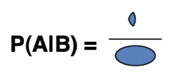
Now let’s consider the conditional probability \(P(A \mid B)\), which is said “probability of \(A\) given \(B\)”. We know that the dart hit \(B\), so the denominator is no longer the entire sample space \(\Omega\) (the rectangle). Instead, it the denominator is \(B\). Similarly, the numerator is no longer all of \(A\), because some parts of \(A\) aren’t also in \(B\). Instead, the numertor is the intersection \(A \cap B\). We can visualize this as:
We will extend this visual representation in the section on Bayes’ Theorem.
Visualizing conditional distributions for continuous data
Consider the arbitrary joint distribution \(p_{XY}(X,Y)\) shown below
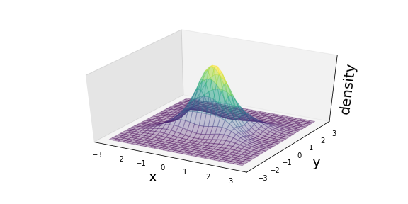
Fig. 8 A schematic of the joint \(p(X,Y)\)
If we want to condition on the random varaible \(Y\) taking on the value \(y=-1.15\), then the conditional distribution \(p_{X\mid Y}(X|Y)\) is just a normalized version of a slice through the joint:
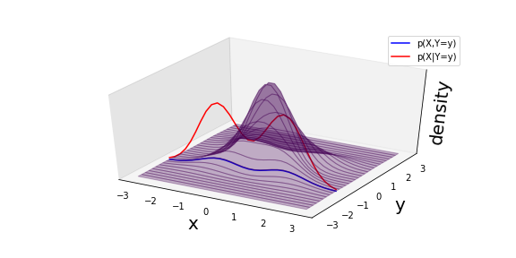
Fig. 9 A schematic of the slice through the joint \(p(X,Y=y)\) and the normalized conditional \(p(X|Y)\).
Similarly, if we want to condition on the random varaible \(X\) taking on the value \(x=1.75\), then the conditional distribution \(p_{Y\mid X}(Y|X)\) is just a normalized version of a slice through the joint:
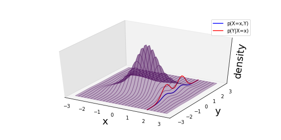
Fig. 10 A schematic of the slice through the joint \(p(X=x,Y)\) and the normalized conditional \(p(Y|X)\).
Note
Here’s a link to the notebook I used to make these images in case it is useful.
Marginal Distributions
The normalization factors in the denominator of Equations (1) and (2) involve probability distributions over an individual variables \(p_X(X)\) or \(p_Y(Y)\) without conditioning on the other. These are called marginal distributions and they correspond to integrating out (or marginalizing) the other variable(s). Eg.
In many ways, marginalization is the opposite of conditioning.
For high dimensional problems, marginalization is difficult as it involves high dimensional integrals. Naive numerical integration is often not tractable, which has motivated a number of different approaches to approximate the integrals, such as Monte Carlo integration.
Chain Rule of Probability
One very powerful and useful result is that, without loss of generality, one can decompose a joint distribution into the appropriate product of conditionals. For example, one can always write the joint distribution for \(X\) and \(Y\) as
Similarly, one can always decompose the the joint for three variables as
And this type of decomposition for the joint for \(N\) random variables \(X_1, \dots, X_N\) is often written in this way:
Note that here I’ve added subscripts to the distributions as they are all different in general. In some cases, one uses this same kind of decomposition and additionally assumes that there is some structure across the different distributions (eg. in a Markov process or an autoregressive model).
An alternative notation that is often found is:
where the first term \(p(X_{1})\) without any conditioning is implied.
A more general formulation
The formulation of the chairn rule See Theorem 1.2.2 (Chain rule) in the NYU CDS lecture notes on Probability and Statistics for a more general formulation
A mnemonic on conditional distributions: Units
We will see many different types of conditional distributions in this course, and manipulating them can be error prone and confusing. Manipulating conditional distributions takes some practice, it is not much different than learning to manipulate upper- and lower-indices in special realtivity and Einstein notation. As we will see later, some distributions have additional structure – some variables may be (assmed to be) independent or conditionally independent – and in these cases the decomposition isn’t completely general, but it there are still some rules.
For example, I know that \(p(X,Y|Z)p(X)\) is not a valid decomposition of any joint \(p(X,Y,Z)\) or conditional \(p(X,Y|Z)\). I know this immediately by inspection because the \(X\) appears on the left of the \(\mid\) more than once. If \(X,Y,Z\) are continuous and have units, then the units of this expression would be \([Y]^{-1}[X]^{-2}\). Similarly, if I wanted to check that it was normalized I would want to integrate it. While I can assume \(\int p(x,y|z) dx dy= 1\) and \(\int p(x) dx = 1\), there is no reason for \(\int p(x,y|z)p(x)\) will be 1, and it will still have units of \([X]^{-1}\).
Personally, I like to sort the terms like this \(p(X,Y) = p(X|Y) p(Y)\) instead of like this \(p(X,Y) = p(Y) p(X|Y)\). Or like this \(P(A \cap B) = P(A \mid B) p(B)\) instead of like this \(P(A \cap B) = p(B) P(A \mid B)\). In both cases, what one can form a joint distribution by starting with a conditioanl and then multiplying by a distribution for what is being conditioned on. I find that putting the terms in this order helps me avoid mistakes and it’s easier to connect to the chian rule of probability.