Revisiting error propagation with automatic differentiation
By Kyle Cranmer, March 2, 2020
This notebook is dedicated to Feeman Dyson, who died on February 28, 2020 in Princeton, NJ at the age of 96.
“New directions in science are launched by new tools much more often than by new concepts. The effect of a concept-driven revolution is to explain old things in new ways. The effect of a tool-driven revolution is to discover new things that have to be explained.”
– Freeman Dyson
)
Reminder of propagation of errors
This notebook was made to investigate the propagation of errors formula. We imagine that we have a function \(q(x,y)\) and we want to propagate the uncertainty on \(x\) and \(y\) (denoted \(\sigma_x\) and \(\sigma_y\), respectively) through to the quantity \(q\).
The most straight forward way to do this is just randomly sample \(x\) and \(y\), evaluate \(q\) and look at it’s distribution. This is really the definition of what we mean by propagation of uncertianty. It’s very easy to do with some simply python code.
The calculus formula for the propagation of errors is really an approximation. This is the formula for a general \(q(x,y)\)
In the special case of addition \(q(x,y) = x\pm y\) we have \(\sigma_q^2 = \sigma_x^2 + \sigma_y^2\).
In the special case of multiplication \(q(x,y) = x y\) and division \(q(x,y) = x / y\) we have \((\sigma_q/q)^2 = (\sigma_x/x)^2 + (\sigma_y/y)^2\), which we can rewrite as \(\sigma_q = (x/y) \sqrt{(\sigma_x/x)^2 + (\sigma_y/y)^2}\)
Let’s try out these formulas and compare the direct approach of making the distribution to the prediction from these formulas
Automatic Differentiation
Excerpts from the Wikipedia article: https://en.wikipedia.org/wiki/Automatic_differentiation
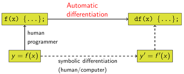
In mathematics and computer algebra, automatic differentiation (AD), also called algorithmic differentiation or computational differentiation,[1][2] is a set of techniques to numerically evaluate the derivative of a function specified by a computer program. AD exploits the fact that every computer program, no matter how complicated, executes a sequence of elementary arithmetic operations (addition, subtraction, multiplication, division, etc.) and elementary functions (exp, log, sin, cos, etc.). By applying the chain rule repeatedly to these operations, derivatives of arbitrary order can be computed automatically, accurately to working precision, and using at most a small constant factor more arithmetic operations than the original program.

Usually, two distinct modes of AD are presented, forward accumulation (or forward mode) and reverse accumulation (or reverse mode). Forward accumulation specifies that one traverses the chain rule from inside to outside (that is, first compute \({\displaystyle dw_{1}/dx}\) and then \({\displaystyle dw_{2}/dw_{1}}\) and at last \({\displaystyle dy/dw_{2}})\), while reverse accumulation has the traversal from outside to inside (first compute \({\displaystyle dy/dw_{2}}\) and then \({\displaystyle dw_{2}/dw_{1}}\) and at last \({\displaystyle dw_{1}/dx})\). More succinctly,
forward accumulation computes the recursive relation: \({\displaystyle {\frac {dw_{i}}{dx}}={\frac {dw_{i}}{dw_{i-1}}}{\frac {dw_{i-1}}{dx}}}\) with \({\displaystyle w_{3}=y}\), and,
reverse accumulation computes the recursive relation: \({\displaystyle {\frac {dy}{dw_{i}}}={\frac {dy}{dw_{i+1}}}{\frac {dw_{i+1}}{dw_{i}}}}\) with \({\displaystyle w_{0}=x}\).
We will use https://jax.readthedocs.io/en/latest/notebooks/autodiff_cookbook.html
from jax import grad, jacfwd
import jax.numpy as np
Now here are 3 lines of code for the propagation of uncertainty formula
def error_prop_jax_gen(q,x,dx):
    jac = jacfwd(q)
    return np.sqrt(np.sum(np.power(jac(x)*dx,2)))
Setup two observations with uncertainties
Below I’ll use \(x\) and \(y\) for symbols, but they will be stored in the array x so that x[0]=\(x\) and `x[1]=\(y\).
x_ = np.array([2.,3.])
dx_ = np.array([.1,.1])
/Users/cranmer/anaconda3/envs/jax-md/lib/python3.6/site-packages/jax/lib/xla_bridge.py:120: UserWarning: No GPU/TPU found, falling back to CPU.
  warnings.warn('No GPU/TPU found, falling back to CPU.')
Addition and Subtraction
In the special case of addition \(q(x,y) = x\pm y\) we have \(\sigma_q^2 = \sigma_x^2 + \sigma_y^2\).
def q(x):
    return x[0]+x[1]
def error_prop_classic(x, dx):
    # for q = x[0]*x[1]
    ret = dx[0]**2 + dx[1]**2
    return np.sqrt(ret)
print('q = ', q(x_), '+/-', error_prop_classic(x_, dx_))
q = 5.0 +/- 0.14142136
print('q = ', q(x_), '+/-', error_prop_jax_gen(q, x_, dx_))
q = 5.0 +/- 0.14142136
Multiplication and Division
In the special case of multiplication
and division
which we can rewrite as
def q(x):
    return x[0]*x[1]
def error_prop_classic(x, dx):
    # for q = x[0]*x[1]
    ret = (dx[0]/x[0])**2 + (dx[1]/x[1])**2
    return (x[0]*x[1])*np.sqrt(ret)
print('q = ', q(x_), '+/-', error_prop_classic(x_, dx_))
q = 6.0 +/- 0.36055514
print('q = ', q(x_), '+/-', error_prop_jax_gen(q, x_, dx_))
q = 6.0 +/- 0.36055514
def q(x):
    return x[0]/x[1]
def error_prop_classic(x, dx):
    # for q = x[0]*x[1]
    ret = (dx[0]/x[0])**2 + (dx[1]/x[1])**2
    return (x[0]/x[1])*np.sqrt(ret)
print('q = ', q(x_), '+/-', error_prop_classic(x_, dx_))
q = 0.6666667 +/- 0.040061682
print('q = ', q(x_), '+/-', error_prop_jax_gen(q, x_, dx_))
q = 0.6666667 +/- 0.040061682
Powers
\(q(x,y) = x^m y^n\) we have
which we can rewrite as
def q(x, m=2, n=3):
    return np.power(x[0],m)*np.power(x[1],n)
x_ = np.array([1.5, 2.5])
dx_ = np.array([.1, .1])
q(x_)
DeviceArray(35.15625, dtype=float32)
def error_prop_classic(x, dx):
    # for q = x[0]*x[1]
    dq_ = q(x_)*np.sqrt(np.power(2*dx_[0]/x_[0],2)+np.power(3*dx_[1]/x_[1],2))
    return dq_
print('q = ', q(x_), '+/-', error_prop_classic(x_, dx_))
q = 35.15625 +/- 6.3063865
print('q = ', q(x_), '+/-', error_prop_jax_gen(q, x_, dx_))
q = 35.15625 +/- 6.3063865
Misc Examples
See some examples here:
http://www.geol.lsu.edu/jlorenzo/geophysics/uncertainties/Uncertaintiespart2.html
Example: w = (4.52 ± 0.02) cm, A = (2.0 ± 0.2), y = (3.0 ± 0.6) cm. Find
The second relative error, (Dy/y), is multiplied by 2 because the power of y is 2.
The third relative error, (DA/A), is multiplied by 0.5 since a square root is a power of one half.
So Dz = 0.49 (28.638 ) = 14.03 which we round to 14
z = (29 ± 14) Using Eq. 3b, z=(29 ± 12) Because the uncertainty begins with a 1, we keep two significant figures and round the answer to match.
def q(x):
    return x[0]*x[2]*x[2]/np.sqrt(x[1])
x_ = np.array([4.52, 2., 3.]) #w,A,y
dx_ = np.array([.02, .2, .6])

print('q = ', q(x_), '+/-', error_prop_jax_gen(q, x_, dx_))
q = 28.765104 +/- 11.596283
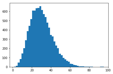
Check with a plot
import numpy as onp  #using jax as np right now
w_ = onp.random.normal(x_[0], dx_[0], 10000)
A_ = onp.random.normal(x_[1], dx_[1], 10000)
y_ = onp.random.normal(x_[2], dx_[2], 10000)
x__ = np.vstack((w_, A_, y_))
z_ = q(x__)
print('mean =', np.mean(z_), 'std = ', np.std(z_))
mean = 30.050316 std = 11.813263
import matplotlib.pyplot as plt
_ = plt.hist(z_, bins=50)

Example 2
also taken from http://www.geol.lsu.edu/jlorenzo/geophysics/uncertainties/Uncertaintiespart2.html
w = (4.52 ± 0.02) cm, x = (2.0 ± 0.2) cm, y = (3.0 ± 0.6) cm.
Find
We have v = wx = (9.0 ± 0.9) cm.
The calculation of the uncertainty in is the same as that shown to the left. Then from Eq. 1b
Dz = 3.7
z = (18 ± 4) .
def q(x):
    # [w,x,y]
    return x[0]*x[1]+x[2]*x[2]
x_ = np.array([4.52, 2., 3.]) #w,x,y
dx_ = np.array([.02, .2, .6])
print(q(x_),'+/-', error_prop_jax_gen(q, x_, dx_))
18.04 +/- 3.711983
An example with many inputs
The code we used for error_prop_jax_gen is generic and supports functions q on any number of variables
def q(x):
    return np.sum(x)
x_ = 1.*np.arange(1,101) #counts from 1-100 (and 1.* to make them floats)
dx_ = 0.1*np.ones(100)
The sum from \(1 to N\) is \(N*(N+1)/2\) (see the story of Gauss), so we expect q(x)=5050. And the uncertainty should be \(\sqrt{100}*0.1\) = 1.
print(q(x_),'+/-', error_prop_jax_gen(q, x_, dx_))
5050.0 +/- 1.0
another toy example… product from 1 to 10
def q(x):
    return np.product(x)
x_ = 1.*np.arange(1,11) #counts from 1-100 (and 1.* to make them floats)
dx_ = 0.1*np.ones(10)
print(q(x_),'+/-', error_prop_jax_gen(q, x_, dx_))
3628800.0 +/- 451748.1
Checking this is an exercise left to the reader :-)
