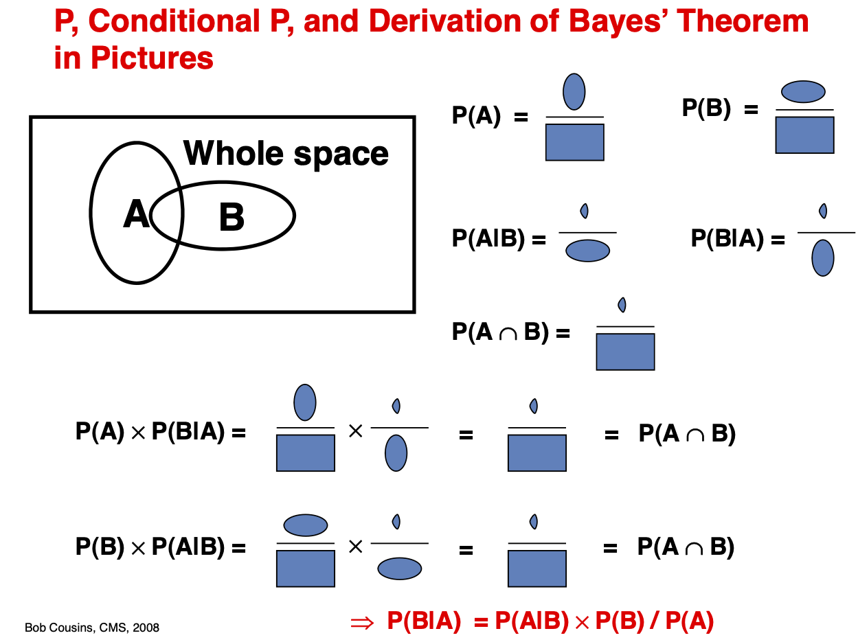
Bayes’ Theorem
Earlier we discussed conditional probability for an event \(A\) given another event \(B\): \(P(A \mid B)\). Examples:
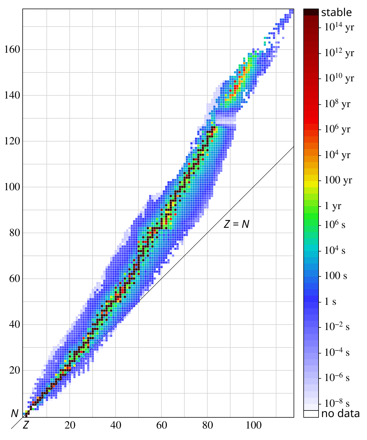
the probability to have \(N\) neutrons in an atom given an atomic number of \(Z\) plot
the distribution of height \(h\) given that you are a professional basketball player
the disribution of some generic data \(X\) given a theory with parameters \(\theta\)
the probability of testing negative for COVID19 given that you actually have COVID19
Bayes’ rule allows us to invert the relationship from \(P(A \mid B)\) to \(P(B \mid A)\). It can also be thought of as updating our prior probability for \(B\) to a posterior probability for \(B\) given that we observe \(A\).
Theorem (Bayes’ rule)
For any events \(A\) and \(B\) in a probability space \((\Omega,\mathcal{F},P)\)
as long as \(P (A) > 0\).
In our examples this would turn into:
the probability for an atom to have an atomic number of \(Z\) given that it has \(N\) neutrons
the probability to be a professional basketball player given your height is \(h\)
the probability disribution for a theory’s parameters \(\theta\) given data \(X\)
the probability of actually having COVID19 given that you tested negative for COVID19
Breaking down the terms
Each of the terms in Bayes’ rule has a name and interpretation. For this I think it is useful to think not of generic \(A\) and \(B\), but to think of some theory of the Universe with parameters \(\theta\) (like the Higgs mass or the cosmological constant) and the predictions for what the data \(X\) would look like given \(\theta\). Then Bayes Rule is
\(p(X \mid \theta)\): the likelihood: the probability distributon of the data \(X\) given the theoretical parameters \(\theta\)
\(p(\theta)\): the prior probability for the parameter \(\theta\)
\(p(\theta \mid X)\): the posterior probability of \(\theta\) given \(X\)
\(p(X)\): the normalizing constant often referred to as the evidence.
An example:
To be concrete, consider this plot from the ATLAS experiment at the Large Hadron Collider from July 2012. It shows the distribution of a random variable \(m_{4l}\)) given three different hypothesized Higgs boson masses \(m_H=(125, 150, 190)\) GeV. You can think of the data as \(\{m_{4l}\}=X\) and the parameter as \(m_H=\theta\).
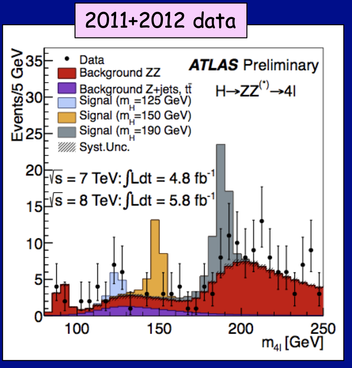
Fig. 12 A plot from the ATLAS experiment at the Large Hadron Collider from July 2012. It shows histograms for the observed data (black dots) as well as the expected distribution for a random variable denoted \(m_{4l}\) given different hypothesized Higgs boson basses \(m_H\) (blue, orange, grey, which are stacked on top of the common \(m_H\)-independent backgrounds red+purple).
If we ask ourselves, what is the probability distribution for the Higgs mass given the data \(p(m_H \mid \{ m_{4l}\} )\) Bayes theorem tells us we need the likelihood \(p(\{m_{4l}\} \mid m_H)\), which we can calculate using Quantum Field Theory and the prior probability \(p(m_H)\). But where does \(p(m_H)\) come from? We cannot calculate that from Quantum Field Theory, it is simply a parameter of the theory. If we were to say that our prior \(p(m_H)\) is informed by some other experimental evidence \(Y\), and it is really a posterior \(p(m_H \mid Y)\), we would just find ourselves in the same situation for that previous measurement. Eventually we will be led to some original prior on \(m_H\), which is not supported by experimental evidence or theoretical argument. More over, if we define probability in as the frequency that an event occurs in a large number of trials, what is the ensemble of trials? These would correspond to different universes. That interpretation may be ok if you embrace the idea of the Multiverse (in fact, this is at the heart of the anthropic principle), but if you imagine a single universe with an unknown true value for \(m_H\), then \(p(m_H)\) is simply not defined and it makes no sense to talk about a prior or a posterior on the parameter.
Axioms of probability
It may be surprising to first learn that there is not a unique definition of probability given how mathematical and formal probability and statistics are. There are two main “schools” usually refered to as Frequentist and Bayesian statistics. Frequentists do not deny that Bayes’ theorem is true – it’s a thoerem after all – but they do define probability in terms of the limit of long term frequency of an event occuring in multiple trials and, therefore, deny assigning probabilities to some quantities. Eg. the Higgs boson mass \(m_H\) is not a random variable, but simply a parameter that indexes (or parameterizes) of a family of distributions. In contrast, Bayesians tend to promote these parameters to random variables with corresponding probability distributions. How is this probability defined? There are many potential interpretations of probability, but a common interpretation for Bayesian statistics is a subjective degree of belief. It may seem surprising that one could use a subjective degree of belief in such a mathematical topic, but the formal mathematics of probability and statistics is sound as long as the probability function (or measure) \(P\) in the probability space \((\Omega, \mathcal{F}, P)\) satisfies Kolmogorov’s axioms of probability (see also Stanford Encyclopedia of Philosophy). We saw these axioms when we first introduced random variables.
The frequentist definition of probability in terms of limiting frequency of events across many trials satisfies Kolmogorov’s axioms (see criticism here). But how do you quantify subjective degree of belief? There is a nice article in the Stanford Encyclopedia of Philosophy, which I will quote from:
Subjective probabilities are traditionally analyzed in terms of betting behavior. Here is a classic statement by de Finetti (1980):
Let us suppose that an individual is obliged to evaluate the rate p at which he would be ready to exchange the possession of an arbitrary sum \(S\) (positive or negative) dependent on the occurrence of a given event \(E\), for the possession of the sum \(pS\); we will say by definition that this number \(p\) is the measure of the degree of probability attributed by the individual considered to the event \(E\), or, more simply, that \(p\) is the probability of \(E\) (according to the individual considered; this specification can be implicit if there is no ambiguity).
This boils down to the following analysis:
Your degree of belief in \(E\) is \(p\) iff \(p\) units of utility is the price at which you would buy or sell a bet that pays 1 unit of utility if \(E\), 0 if not \(E\).
A Dutch book (against an agent) is a series of bets, each acceptable to the agent, but which collectively guarantee her loss, however the world turns out. Ramsey notes, and it can be easily proven (e.g., Skyrms 1984), that if your subjective probabilities violate the probability calculus, then you are susceptible to a Dutch book. For example, suppose that you violate the additivity axiom by assigning \(P(A \cup B) < P(A) + P(B)\), where A and B are mutually exclusive. Then a cunning bettor could buy from you a bet on \(A \cup B\) for \(P(A \cup B)\) units, and sell you bets on \(A\) and \(B\) individually for \(P(A)\) and \(P(B)\) units respectively. He pockets an initial profit of \(P(A) + P(B) - P(A \cup B)\), and retains it whatever happens. Ramsey offers the following influential gloss: “If anyone’s mental condition violated these laws [of the probability calculus], his choice would depend on the precise form in which the options were offered him, which would be absurd.” (1980, 41)
Equally important, and often neglected, is the converse theorem that establishes how you can avoid such a predicament. If your subjective probabilities conform to the probability calculus, then no Dutch book can be made against you (Kemeny 1955); your probability assignments are then said to be coherent. In a nutshell, conformity to the probability calculus is necessary and sufficient for coherence.