Covariance and Correlation
Variance for a single variable
The expected value or mean of a random variable is the first moment, analogous to a center of mass for a rigid body. The variance of a single random variable is the second moment: it is the expectation of the squared deviation of a random variable from its mean. It is analogous to the moment of inertia about the center of mass.
where \(\mu = \mathbb{E}[X]\)
The units of \(\operatorname{Var} (X)\) are \([\operatorname{Var} (X)] = [X]^2\). For that reason, it is often more intuitive to work with the standard deviation of \(X\), usually denoted \(\sigma_X\), which is the square root of the variance:
In statistical mechanics, you may have seen notation like this: \(\sigma_X = \sqrt{ \left\langle \left( X - \langle X \rangle \right)^2 \right\rangle }\)
Covariance
When dealing with multivariate data, the notion of variance must be lifted to the concept of covariance. Covariance captures how one variable deviates from its mean as another variable deviates from it’s mean. Say we have two variables \(X\) and \(Y\), then the covariance for the two variables is defined as
If \(X\) is on average greater than its mean when \(Y\) is greater than its mean (and, similarly, if \(X\) is on average less than its mean when \(Y\) is less than its mean), then we say the two variables are positively correlated. In the opposit case, when \(X\) is on average less than its mean when \(Y\) is greater than its mean (and vice versa), then we say the two variables are negatively correlated. If \(\operatorname{Cov}(X,Y) = 0\), then we say the two variables are uncorrelated.
A useful identity
Correlation coefficient
The covariance \(\operatorname{Cov}(X,Y)\) has units \(([X][Y])^{-1}\), and thus depends on the units for \(X\) and \(Y\). It is desireable to have a unitless measure of how “correlated” the two variables are. One way to do this is through the Correlation coefficient \(\displaystyle \rho _{X,Y}\), which simply divides out the standard deviation of \(X\) and \(Y\)
where \(\sigma_X^2 = \textrm{cov}(X,X)\) and \(\sigma_Y^2 = \textrm{cov}(Y,Y)\)
Warning
It is common to mistakenly think that if two variables \(X\) and \(Y\) are “uncorrelated” that they are statistically independent, but this is not the case. It is true that if two variables \(X\) and \(Y\) are “correlated” (have non-zero covariance), then the two variables are statistically dependent, but the converse is not true in general. We will see this in our Simple Data Exploration.
Covariance matrix
When dealing with more than two variables, there is a straightforward generalization of covariance (and correlation) in terms of a covariance matrix 1. Given random variables \(X_1, \dots, X_N\), the covariance matrix is an \(N\times N\) matrix whose \((i,j)\) entry is the covariance
If the entries are represented as a column vector \({\displaystyle \mathbf {X} =(X_{1},X_{2},...,X_{n})^{\mathrm {T} }}\), then the covariance matrix can be written as
with \({\displaystyle \mathbf {\mu _{X}} =\mathbb{E} [\mathbf {X} ]}\) also represented as a column vector.
Note
The inverse of this matrix, \({\displaystyle \operatorname {K} _{\mathbf {X} \mathbf {X} }^{-1}}\), if it exists, is also known as the concentration matrix or precision matrix.
Correlation Matrix
An entity closely related to the covariance matrix is the correlation matrix 1,
Each element on the principal diagonal of a correlation matrix is the correlation of a random variable with itself, which always equals 1.
Equivalently, the correlation matrix can be written in vector-matrix form as
where \({\displaystyle \operatorname {diag} (\operatorname {K} _{\mathbf {X} \mathbf {X} })}\) is the matrix of the diagonal elements of \({\displaystyle \operatorname {K} _{\mathbf {X} \mathbf {X} }}\) (i.e., a diagonal matrix of the variances of \(X_{i}\) for \(i=1,\dots ,n)\).
Visualizing covariance as an ellipse
Often an ellipse is used to visualize a covariance matrix, but why? This is only well-motivated if one expects the data to be normally distributed (aka Gaussian distributed). This is because the contours of a 2-d normal are ellipses, and in higher dimensions the contours are ellipsoids.
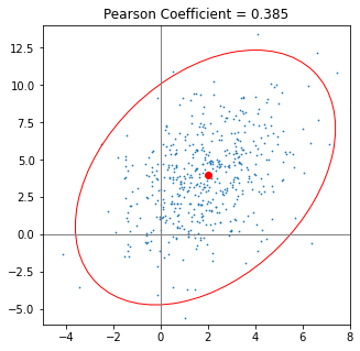
Fig. 13 width: 30%
A scatter plot of two correlated, normally-distributed variables and the error ellipse from An Alternative Way to Plot the Covariance Ellipse by Carsten Schelp.
Consider a random variable \(X\) that is distributed as a multivariate normal (aka multivariate Gaussian) distribution, e.g. \({\displaystyle \mathbf {X} \ \sim \ {\mathcal {N}}({\boldsymbol {\mu }},\,{\boldsymbol {\Sigma }}})\), where \(\boldsymbol{\mu}\) is the multivariate mean and \(\Sigma\) is the covariane matrix. The probability density for the multivariate normal is given by
The contours correspond to values of \(\mathbf{X}\) where \(({\mathbf {x} }-{\boldsymbol {\mu }})^{\mathrm {T} }{\boldsymbol {\Sigma }}^{-1}({\mathbf {x} }-{\boldsymbol {\mu }}) = \textrm{Constant}\).
Understanding the geometry of this ellipse requires the linear algebra of the covariance matrix, and it’s a useful excercise to go through:
This notebook is duplicated from the repository linked to in this article: An Alternative Way to Plot the Covariance Ellipse by Carsten Schelp, which has a GPL-3.0 License.
This is also a nice page
With empirical data
We can estimate the covariance of the parent distribution \(p_{XY}\) with the sample covariance, using the sample mean in place of the expectation \(\mathbb{E}_{p_X}\).
As we will see in our Simple Data Exploration and Visualizing joint and marginal distributions, the sample covariance and correlation matrices can be conveniently computed for a pandas dataframe with dataframe.cov() and dataframe.corr()
- 1(1,2)
Adapted from Wikipedia article on Covariance Matrix