Transformation of likelihood with change of random variable¶

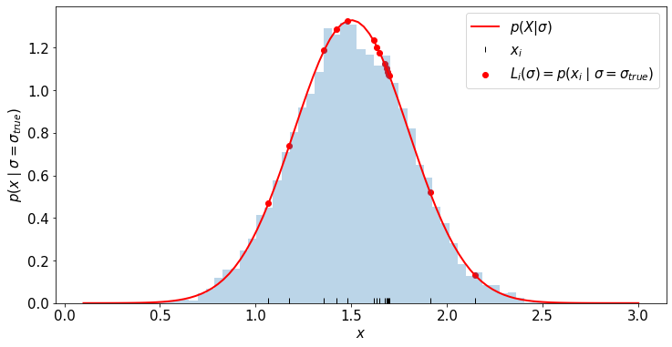
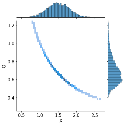
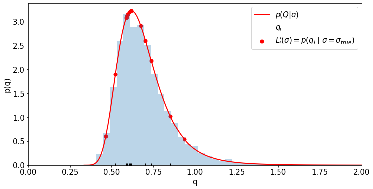
In this notebook we will be looking at how the likelihood and likelihood ratio transform under a change of variables for the random variable. In particular we will consider \(X\sim P_X(X|\sigma) := N(\mu=1,\sigma)\) and \(Q = 1/X\). We will also use automatic differentiation to calculate \(P_Q(Q|\sigma)\).

by Kyle Cranmer, September 16, 2020

import numpy as np
from scipy.stats import norm
import matplotlib.pyplot as plt
from matplotlib import rcParams
rcParams.update({'font.size': 15})
#rcParams.update({'font.size': 18,'text.usetex': True})
rcParams['figure.figsize'] = 12,6

true_sigma=0.3
true_mean = 1.5
N = 10000

def my_family_of_pdfs_for_X(x, sigma):
    #return 1./np.sqrt(2.*np.pi)/sigma * np.exp( -(x-mu)**2/2/sigma**2 )
    return norm.pdf(x,loc=true_mean, scale=sigma)

# Generate a lot of synthetic data for visualizing distribution 
x_for_hist = np.random.normal(true_mean, true_sigma, N)

# Generate a small synthetic data set
x_for_data = norm.rvs(loc=true_mean, scale=true_sigma, size=15)
x_for_data

array([1.67412528, 1.61534283, 1.911109  , 1.69040415, 1.64757904,
       2.14665653, 1.68322071, 1.48080159, 1.17534116, 1.69543711,
       1.42219525, 1.06666355, 1.35731658, 1.63379274, 1.69843078])

x_for_plot = np.linspace(0.1,3,100)

likelihood_i = my_family_of_pdfs_for_X(x_for_data, true_sigma)

_ = plt.hist(x_for_hist, bins=50, density=True, alpha=.3)
plt.plot(x_for_plot, my_family_of_pdfs_for_X(x_for_plot, true_sigma), c='r', label=r'$p(X|\sigma)$',lw=2)
plt.scatter(x_for_data, likelihood_i, c='r', label=r'$L_i(\sigma) = p(x_i \mid \sigma=\sigma_{true})$')
plt.plot(x_for_data, [0.01]*len(x_for_data), '|', color='k', label=r'$x_i$')
plt.xlabel(r'$x$')
plt.ylabel(r'$p(x \mid \sigma=\sigma_{true}$)')
plt.legend()

<matplotlib.legend.Legend at 0x7ffe50521f40>

../_images/likelihood-change-obs_8_1.png

def q(x):
    return 1/x

q_for_hist = q(x_for_hist)
q_for_plot = q(x_for_plot)
q_for_data = q(x_for_data)

from jax import grad, vmap
import jax.numpy as np

#define the gradient with grad(q)
dq = vmap(grad(q))  #dq is a new python function
print(dq(np.array([.5]))) # should be -4

[-4.]

/Users/cranmer/anaconda3/envs/stats-book-2/lib/python3.8/site-packages/jax/lib/xla_bridge.py:130: UserWarning: No GPU/TPU found, falling back to CPU.
  warnings.warn('No GPU/TPU found, falling back to CPU.')

def my_family_of_pdfs_for_Q(q, sigma):
    #use change of variables formua
    x = 1/q
    base_pdf = my_family_of_pdfs_for_X(x, sigma)
    jacobian = np.abs(dq(x))
    return base_pdf/jacobian

import seaborn as sns

a_plot = sns.jointplot(x=x_for_hist, y=q_for_hist, kind="hist", fill=True)
a_plot.ax_marg_y.set_ylim(0.25, 1.25)
a_plot.set_axis_labels('X', 'Q', fontsize=16)

<seaborn.axisgrid.JointGrid at 0x7ffe5088c220>

../_images/likelihood-change-obs_15_1.png

_ = plt.hist(q_for_hist, bins=np.linspace(0,2,50), density=True, alpha=.3)
plt.plot(q_for_plot, my_family_of_pdfs_for_Q(q_for_plot, true_sigma), c='r', lw=2, label=r'$p(Q|\sigma)$')
plt.scatter(q_for_data, my_family_of_pdfs_for_Q(q_for_data, true_sigma), c='r', lw=2, label=r'$L^\prime_i(\sigma) = p(q_i \mid \sigma=\sigma_{true})$')
plt.plot(q_for_data, [0.01]*len(q_for_data), '|', color='k', label=r'$q_i$')
plt.xlim((0,2))
plt.xlabel('q')
plt.ylabel('p(q)')
plt.legend()

<matplotlib.legend.Legend at 0x7ffe32f4ef70>

../_images/likelihood-change-obs_16_1.png

def my_X_likelihood(data,sigma):
    L = 1.
    for x in data:
        L *= my_family_of_pdfs_for_X(x,sigma)
    return L

'''
import numpy as np
def my_Q_likelihood(data,sigma):
    """This is a plane native python way to return array of likelihood values for each sigma"""
    ret = 0.*sigma
    for i, s in enumerate(sigma):
        ret[i] = np.prod(my_family_of_pdfs_for_Q(data,s))
    return ret
'''


#import jax.numpy as np
def my_Q_likelihood(data,sigma):
    """this is a faster way of acheiving the above with broadcasting"""
    data_ = np.tile(data, sigma.size)
    sigma_ = np.repeat(sigma, data.size)
    return np.prod(my_family_of_pdfs_for_Q(data_,sigma_).reshape(sigma.size,data.size),axis=1)

sigma_for_plot = np.linspace(.1,1)

x_likelihood = my_X_likelihood(x_for_data, sigma_for_plot)

q_likelihood = my_Q_likelihood(q_for_data, sigma_for_plot)

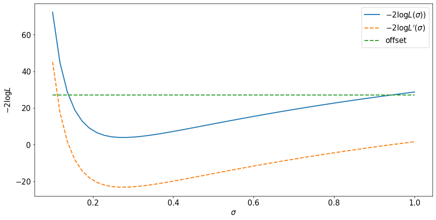
likelihood_offset = -2.*np.log(x_likelihood)[0]+2.*np.log(q_likelihood)[0]
print('observed offset is ', likelihood_offset)

observed offset is  27.105434

def predict_offset_from_jacobian(data):
    return 2*np.sum(np.log(1./np.abs(dq(data))))

print("predicted offset is ", predict_offset_from_jacobian(x_for_data))

predicted offset is  27.105421

fig, ax = plt.subplots(constrained_layout=True)

ax.plot(sigma_for_plot, -2.*np.log(x_likelihood), label=r'$-2 \log L(\sigma))$', lw=2)
ax.plot(sigma_for_plot, -2.*np.log(q_likelihood), label=r'$-2 \log L^\prime(\sigma)$', ls='dashed',lw=2)
ax.plot(sigma_for_plot, np.ones(sigma_for_plot.size)*likelihood_offset, label=r'offset', ls='dashed',lw=2)
ax.set_ylabel(r'$-2 \log L$')
ax.set_xlabel(r'$\sigma$')
ax.legend()

<matplotlib.legend.Legend at 0x7ffe508d1820>

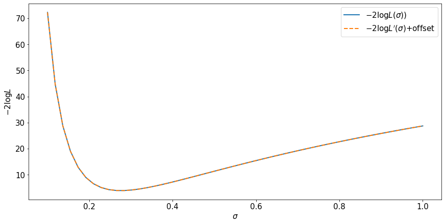
../_images/likelihood-change-obs_23_1.png

fig, ax = plt.subplots(constrained_layout=True)

ax.plot(sigma_for_plot, -2.*np.log(x_likelihood), label=r'$-2 \log L(\sigma))$', lw=2)
ax.plot(sigma_for_plot, -2.*np.log(q_likelihood)+likelihood_offset, label=r'$-2 \log L^\prime(\sigma)$+offset', ls='dashed',lw=2)
ax.set_ylabel(r'$-2 \log L$')
ax.set_xlabel(r'$\sigma$')
ax.legend()

<matplotlib.legend.Legend at 0x7ffe20da6250>

../_images/likelihood-change-obs_24_1.png

Observations¶

The likelihood is not invariant to a change of variables for the random variable because there is a jacobian factor.

The likelihood ratio is invariant to a change of variables for the random variable because the jacobian factors cancel.

The maximum likelihood estimate is invariant.

Regions of the parameter space defined by level sets of the likelihood ratio (or log likelihhood ratio) are invariant.

Statistics and Data Science

Transformation of likelihood with change of random variable¶

Observations¶