This weekend's project was a fun one!

Update: Since the original post I made some more progress. I'm developing the code into my GitHub play/manifoldLearning repository. Below is from the README.

I'm working on a paper about Informtion Geometry.
The first step was an iPython notebook on Visualizing information geometry with multidimensional scaling.

The other python files are me working my way to something more ambitious.

Step 1: The first step is described nicely in this iPython notebook on Visualizing information geometry with multidimensional scaling. Final result shown here. Important part is a grid of points in (μ,σ) being mapped by f:

Step 2: Try various scikit-learn algorithms, setteling on NuSVR. Results not so good, smaller red spots not approximating the larger colorful training samples, particuarly near the edges. The lower-right is what I'm ultimately after, the inverse map of back into the space (μ,σ) -- for these points, that should be a perfect grid. Surprised I can't do regression on

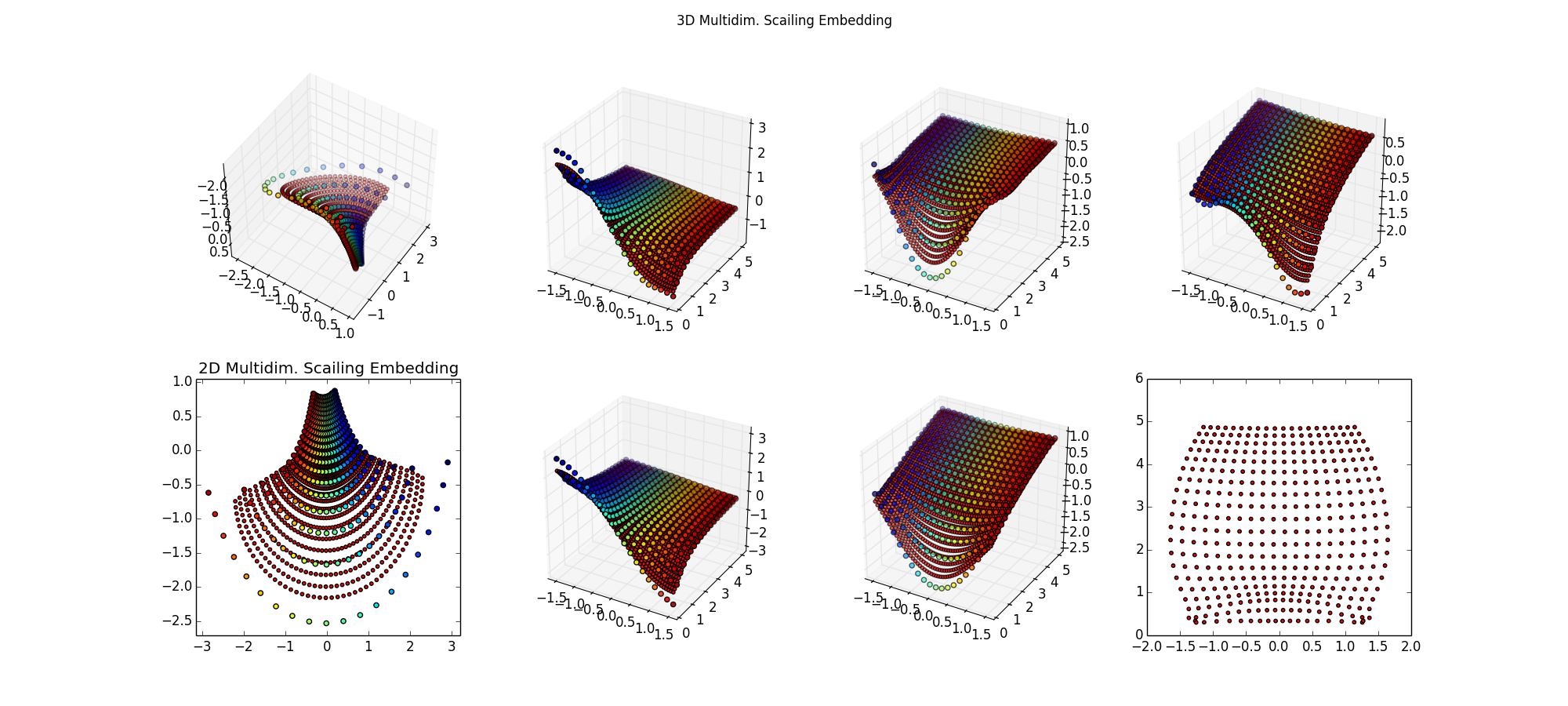
Step 3: Since this is a low dimensional problem with little noise, just try SciPy Interpolation algorithms. Ah, that's better, now I'm getting the grid I want.

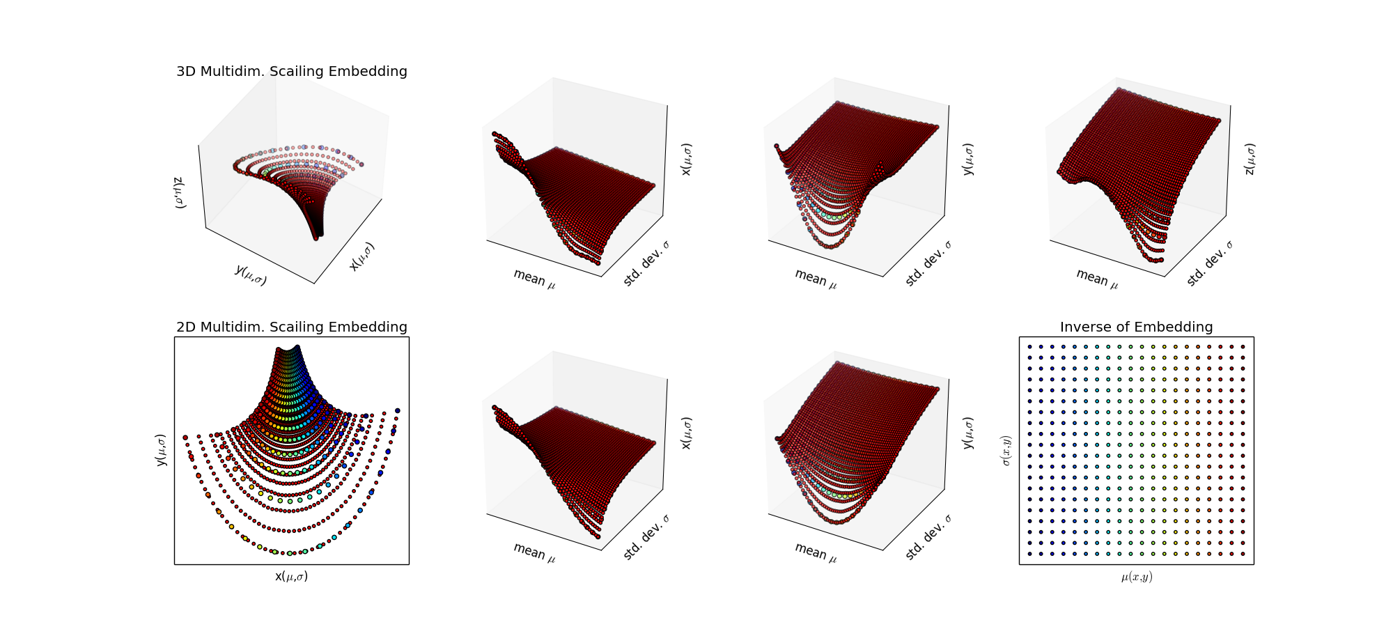
Step 4: To do: make a regular grid in the target space and project it via the inverse into the (μ,σ) plane. This is a "smart" sampling from an information theoretic perspective. It's also a good choice if simulation of the statistical model is expensive (ie. full simulation with GEANT at the LHC, which takes about 20 min per event, and the real collisons are happening at 40 million/sec. )

Step 5: To do: repeat exercise with MSSM SUSY grids published on HepData. Change from Gaussian to Poisson, where I can still solve for the information distance analytically. Repeat steps 3 & 4 for that case, evaluate embedding from information persepctive, and propose a better choice for the parameter scan "grids" used by the ATLAS collaboration.

Step 6: To do: move to a non-number counting model, generate graph of KL distances, use shortest path on this graph (via Dijkstra's algorithm) to approximate the geodesic from the fisher information metric -- perhaps using boost libraries or the code from FINE, amazingly the code is available -- nicely done Kevin Carter!

For convenience, the original notebook is embedded below (using the pelican liquid notebook plugin)

Visualizing information geometry with multidimensional scaling¶

Introduction¶

When I was a graduate student I went to a conference in Germany about neural networks. I didn't know anyone at the conference, and during lunch I joined a Japanese man sitting by himself. We started to chat, and he introduced himself as Shun'ichi Amari. I asked him what he did, and he started to tell me about the fascinating subject of Information Geometry. I had recently studied differential geometry, so I was facinated.

The basic idea is that if you have a parametrized probability model like $G(x|\mu,\sigma)$ one can use ideas from information theory and statistics to define a distance measure (a metric) on the parameter space $(\mu,\sigma)$ that has some nice properties. For example, the distance is invariant to reparametrization of the statistical model (e.g. do I parametrize the distribution in terms of standard devaition $\sigma$ or the variance $\sigma^2$). This last property wouldn't hold if we simply used the Euclidean distance for the parameters $\sqrt{\Delta_1^2 + \Delta_2^2}$.

To me this was very important, because there is some arbitrariness to how we parametrize theories of particle physics, and it's not satisfying when the results depend on that arbitrary choice.

The starting point for informaiton geometry is that one defines the Fisher information metric

\begin{equation} g_{ij}(\vec\alpha) = E\left[ -\partial_i \partial_j \ln L(\vec\alpha) \left | \vec\alpha\right .\right] \end{equation}

This tells you about the geometry of the space locally around the point $\vec\alpha$.

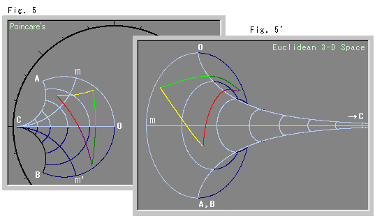
In the case of the Gaussian distribution, the Fisher information metric defines a surface of constant negative curvature. The sphere is the surface of constant positive curvature, so some call this surface of constant negative curvature the pseudo-sphere. Here's an image of the pseudo-sphere from B Jessup

(I can't resist telling the story that the first time I was asked to give a talk at the Institute for Advanced Study, I found myself sitting at lunch next to Juan Maldacena. Juan is the author of the most cited paper in particle physics, which is about -- you guessed it -- a space of constant negative curvature. There I am, a lowly experimental physicist sitting next to one of the greats. He asks me what I'm going to talk about. Despite my better judgement, I tell him that I was going to mention these ideas of information geometry and I tell him the Gaussian example because I thought he'd enjoy that. He looked interested, and asked me "what does the boundary correspond to?" I wasn't sure, but with a little thought I think I could have answered him. Unfortunately, I was so frazled by the fact I had just put myself in that situation that I couldn't think very clearly. Live and learn.)

The project¶

Almost any 2-d Manifold (surface) can be embedded into 3-d in a way that preserves the metric. In the case of the 2-d surface defined by the $(\mu,\sigma)$ of the Gaussian distribution, that embedding into 3-d is the pseudo-sphere I mentioned above. Can we use some numerical algorithms to 'discover' that embedding without ever explicitly figuring out the mapping $(\mu,\sigma) \to \mathbb{R}^3$?

Eventually, what I'd like to do is create some general purpose code that allows me to make these embeddings to visualize the surface based on an arbitrary Fisher information metric $g_{ij}(\vec\alpha)$. That is going to take some more work, because calculating hte distance between points is a bit involved.

In the case of the Gaussian, all of the difficulties of the differential equations that define the geodesic and the integration to define the distance between points can be done analytically. For a "FINE" paper on the subject, look here, in particular eq. 7. There you will find: \begin{equation} D_F(\mu_1,\sigma_1;\mu_2,\sigma_2)) = \sqrt{2}\ln\left[ \frac{ \left| \left(\frac{\mu_1}{\sqrt{2}},\sigma_1\right) +\left(\frac{\mu_2}{\sqrt{2}},-\sigma_2\right) \right| }{ \left| \left(\frac{\mu_1}{\sqrt{2}},\sigma_1\right) -\left(\frac{\mu_2}{\sqrt{2}},-\sigma_2\right) \right| }\right] \end{equation}

Now that I have those distances, I can use the numerical technique of Multidimensional scaling (MDS) to find an embedding that preserves those distances. Luckily, scikit-learn has a nice set of manifold learning algorithms including an MDS implementation. This algorithm only needs to know the distances between pairs of points, and then it will do its best to embed in whatever number of dimensions you ask. Let's see how it does with the Gaussian problem.

First let's get the basics imports out of the way:

In [1]:

%pylab inline

Populating the interactive namespace from numpy and matplotlib

In [2]:

# Author: Kyle Cranmer 
# Licence: BSD

print(__doc__)
import numpy as np

from matplotlib import pyplot as plt
from matplotlib.collections import LineCollection
from mpl_toolkits.mplot3d import Axes3D

from sklearn import manifold
from sklearn.metrics import euclidean_distances
from sklearn.decomposition import PCA

# Next line to silence pyflakes.
Axes3D

Automatically created module for IPython interactive environment

Out[2]:

mpl_toolkits.mplot3d.axes3d.Axes3D

Now let's make a grid in the $(\mu,\sigma)$ plane that is n_samples x n_samples

In [3]:

#make some random samples in 2d
n_samples = 20
seed = np.random.RandomState(seed=3)

#create a set of Gaussians in a grid of mean (-1.5,1.5) and standard devaition (0.2,5)
gridMuSigma=[]
for i in np.linspace(-1.5,1.5,n_samples):
    for j in np.linspace(.2,5,n_samples):
        gridMuSigma.append([i,j])
gridMuSigma=np.array(gridMuSigma)

Now let's code up that handy-dandy distance measure (this would be a big numerical project for an arbitrary metric $g_{ij}(\vec\alpha)$ -- let's takle that later.)

In [4]:

#use 2-d Gaussian information metric for distances
# see equation 7 from http://arxiv.org/abs/0802.2050 ("FINE" paper)
def getDistance(x,y):
    #going to define a measure here
    #print 'in getSim', x, y
    aa = x[0]-y[0]
    ab = x[1]+y[1]
    bb = x[1]-y[1]
    num = np.sqrt((aa**2+ab**2))+np.sqrt((aa**2+bb**2))
    den = np.sqrt((aa**2+ab**2))-np.sqrt((aa**2+bb**2))
    ret = np.log(num/den)
    return ret

Now let's loop through all the pairs of points and calculate the distance between them. For some reason this is referred to as "dissimilarity" in a lot of MDS literature.

In [5]:

# Create the array of "dissimilarities" (distances) between points
tempSim=[]
for x in gridMuSigma:
    temp = []
    for y in gridMuSigma:
        temp.append(getDistance(x,y))
    tempSim.append(temp)
distances=np.array(tempSim)

And now we can use scikit-learn's MDS implementation to embed these points in 3d and 2d so that the euclidean distance between points in the embedding corresponds to the Fisher information distance we calculated above. So even though we start with a 2d grid, the 2d embeddign will not look the same b/c the grid is not uniformly spaced in terms of the information distance.

In [6]:

#make 3d embedding 
mds = manifold.MDS(n_components=3, metric=True, max_iter=3000, eps=1e-9, random_state=seed,
                   dissimilarity="precomputed", n_jobs=1)
embed3d = mds.fit(distances).embedding_

#make 2d embedding
mds2 = manifold.MDS(n_components=2, max_iter=3000, eps=1e-9, random_state=seed,
                   dissimilarity="precomputed", n_jobs=1)
embed2d = mds2.fit(distances).embedding_

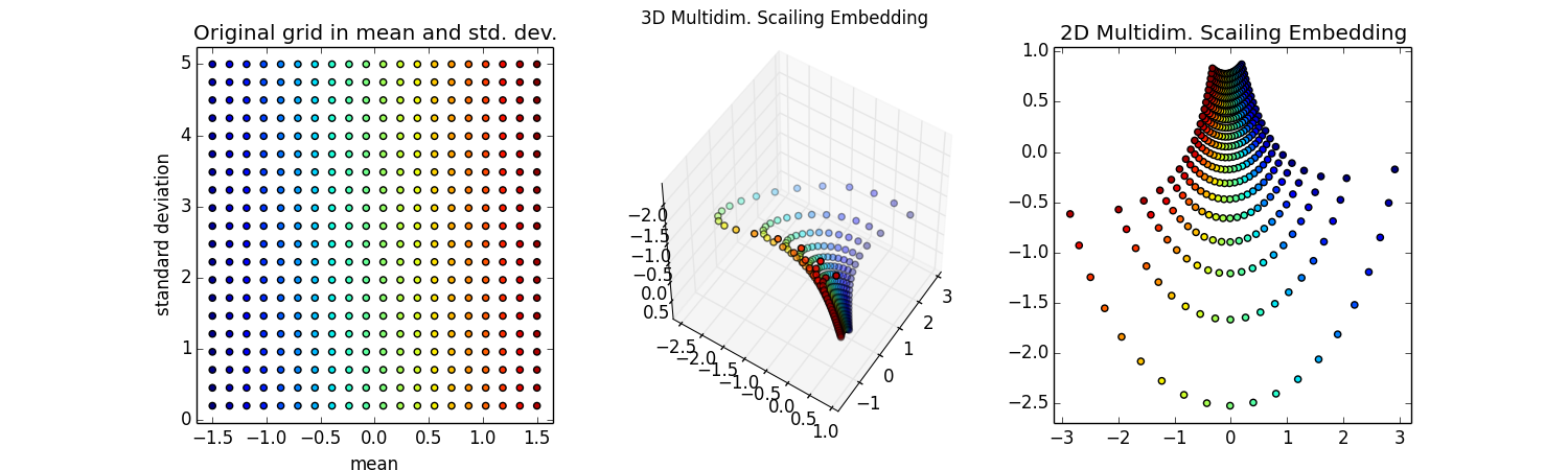
Ok, the hard work is done, now let's make some plots. Let's color each point so we can see the correspondence. The colors will mainly stripe along a constant mean (as in all green points will correspond to a mean of ~0).

In [8]:

#Setup plots
fig = plt.figure(figsize=(5*3,4.5))

# choose a different color for each point
colors = plt.cm.jet(np.linspace(0, 1, len(gridMuSigma)))

#make original grid plot
gridsubpl = fig.add_subplot(131)
gridsubpl.scatter(gridMuSigma[:, 0], gridMuSigma[:, 1], s=20, c=colors)
gridsubpl.set_xlabel('mean')
gridsubpl.set_ylabel('standard deviation')
plt.title('Original grid in mean and std. dev.')
plt.axis('tight')

# plot 3d embedding
#since it is a surface of constant negative curvature (hyperbolic geometry)
#expect it to look like the pseudo-sphere
#http://mathworld.wolfram.com/Pseudosphere.html
subpl = fig.add_subplot(132,projection='3d')
subpl.scatter(embed3d[:, 0], embed3d[:, 1], embed3d[:, 2],s=20, c=colors)
subpl.view_init(42, 101) #looks good when njobs=-1
subpl.view_init(-130,-33)#looks good when njobs=1

plt.suptitle('3D Multidim. Scaling Embedding')
plt.axis('tight')

# plot 2d embedding
subpl2 = fig.add_subplot(133)
subpl2.set_autoscaley_on(False)
subpl2.scatter(embed2d[:, 0], embed2d[:, 1],s=20, c=colors)
plt.title('2D Multidim. Scaling Embedding')
plt.axis('tight')

plt.show()

Wow! Super cool! That looks like the pseudo-sphere!

Ok, it looks like half of the pseudo-sphere. That makes sense because as the means get furhter apart I'm never going to wrap around and have distributions that seem similar.

The 2d embedding looks cool too -- in fact, this image is Fig 5 of the FINE paper](http://arxiv.org/abs/0802.2050) I mentioned above. I'm not quite sure why those authors never made the 3d embedding, but they do have some nice thoughts about how to approximate the Fisher information distance.

You can see some nice correspondence of the curves of constant $\mu$ and constant $\sigma$ between the 2d and 3d embeddings that seem to are reminicent of the correspondance of the pseudosphere and the 2d Poincaré disc model of this same hyperbolic space shown below. The Poincaré disc is 2d, but it is not the same kind of distance-preserving embedding, so that visual correspondance is a bit misleading.

So that was a very fun weekend project. I'm impressed with scikit-learn and how well the MDS algorithm discovered the pseudo-sphere. Now to think about how to visualize some more tricky theoretical physics models where I can describe the information metric, but it's not so easy to calculate the distance between random points in that space.

This post was created entirely in IPython notebook. Download the raw notebook here, or see a static view on nbviewer

Visualizing information geometry with multidimensional scaling¶

Introduction¶

The project¶

Comments