This week NYU hosted a Software Carpentry Bootcamp along with Berkeley and U. Washington (the other institutes in the Moore-Sloan data science environment). I sat in on the python classes (there were also classes in R). However, on Monday, there was a huge announcement from the BICEP2 collaboration about the observation of B-mode polarization in the CMB, which is considered a smoking gun for primordial gravitational waves predicte by inflation. That made it hard to concentrate on python, but I tried to merge the two. I noticed that BICEP2 made their likelihood curve public. I also noticed that they got a bit mixed up with their Bayesian and Frequentist statistics (at least the terminology), so that gave me an idea.
Here's a link to my iPython notebook on alternate BICEP2 error analysis
For convenience, embedded below (using the pelican liquid notebook plugin)
Alternative error analysis for BICEP2 result
Kyle Cranmer kyle.cranmer@nyu.edu Mar 17, 2014
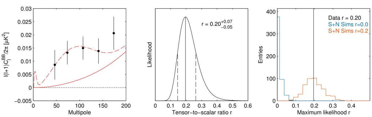
The BICEP2 error quoted on r is 0.2+0.07-0.05 (green below lines), and it looks like it's really a Bayesian shortest interval using a uniform prior on r. Let's see what the error bar looks like by using -2lnL < 1 (intersection of blue and red lines). The likelihood curve is shown here and they made the data public -- thanks BICEP2!
%pylab inline
import requests
import numpy as np
from matplotlib import pyplot as plt
r=requests.get('http://bicepkeck.org/B2_3yr_rlikelihood_20140314.txt')
header = r.text.split('\n')[:12]
Convert the text into an array of floats.
rawLikelihoodData = r.text.split('\n')[13:]
likelihoodScan = []
temp = [i.split('\t') for i in rawLikelihoodData]
temp
for x,y in temp[:-1]:
    likelihoodScan.append([float(x), float(y)])
likelihoodScan = np.array(likelihoodScan)
And the integral is ~1 (so it's like a normalized posterior including the bin width ie. prob/0.001)
np.sum(likelihoodScan[:,1])
Get shortest interval, it will be from [0.145,0.262] to get the 68% for 1$\sigma$
lmax = likelihoodScan[:,1].max()
rpeak = np.where(likelihoodScan[:,1]==lmax)[0][0]
rminBicep, rmaxBicep = rpeak,rpeak
integral,cutoff=0.,lmax-lmax/1000
while integral<0.68:
    rRange = np.where(likelihoodScan[:,1]>cutoff)
    rminBicep=np.min(rRange)
    rmaxBicep=np.max(rRange)
    integral = np.sum(likelihoodScan[rminBicep:rmaxBicep,1])
    cutoff-=lmax/1000
print '[%f, %f]'%( rminBicep, rmaxBicep)
Remake the likelihood curve shown here
plt.plot(likelihoodScan[:,0],likelihoodScan[:,1])
plt.plot(likelihoodScan[rminBicep:rmaxBicep,0],likelihoodScan[rminBicep:rmaxBicep,1],'g')
plt.plot([rminBicep/1000.,rminBicep/1000.],[0.,likelihoodScan[rminBicep,1]],'g')
plt.plot([rmaxBicep/1000.,rmaxBicep/1000.],[0.,likelihoodScan[rmaxBicep,1]],'g')
plt.xlabel('r')
plt.ylabel('Likelihood')

Fortunately, a constant factor on the likelihood cancels out in likelihood ratio (or difference of log likelihoods). So let's see what the typical $\Delta \log L$ or $\Delta \chi^2$ interval would look like.
minLogL = -2 * np.log(np.max(likelihoodScan[:,1]))
rmin, rmax = 0,0
for r, l in likelihoodScan:
    if -2*np.log(l)-minLogL < 1:
        rmin= r
        break

for r, l in likelihoodScan[200:]:
    if -2*np.log(l)-minLogL > 1:
        rmax=r
        break
print '[%f, %f]'%( rmin, rmax)
plt.plot(likelihoodScan[:,0],-2* np.log(likelihoodScan[:,1])-minLogL)
plt.plot([0,0.8],[1.,1.],'r')
plt.plot([rmaxBicep/1000.,rmaxBicep/1000.],[0.,1.],'g')
plt.plot([rminBicep/1000.,rminBicep/1000.],[0.,1.],'g')
plt.plot([rmax,rmax],[0.,1.],'r')
plt.plot([rmin,rmin],[0.,1.],'r')
plt.xlabel('r')
plt.ylabel('-2 ln Likleihood')
plt.ylim([0,2])
plt.xlim([0.1,0.3])

So that's slightly different from the BICEP2 result. In terms of the Bayesian credibility, that interval corresponds to
np.sum(likelihoodScan[147:260,1])
Slightly different numbers and a different probabilistic interpretation, but luckily it doesn't change the profound result.
Assuming that the BICEP2 data are in the asymptotic regieme, then we can quickly estimate the statistical significance of the observation (testing the r=0 hypothesis).
significance = np.sqrt(-2*np.log(likelihoodScan[0,1]))
significance
This was done during a Software Carpentry bootcamp at NYU, it's more of a fun python project than a critique of the BICEP2 result. Congratulations to BICEP2!
Comments
comments powered by Disqus